In the present day scenario, where there is an increasing integration of the financial markets and implementation of various stock market reforms, the activities in the stock market and their relationships with the macro economy have assumed significant importance. In modern economy stock exchange plays a vital role. It can be very helpful to diversify the domestic funds and channels into productive investment, however to perform this significant task it is necessary to study stock market returns and its significant relationship with the macroeconomics variables.

The economists, researchers and policymakers find the association between macroeconomic variables and stock prices very important to study for many reasons. At first, it helps the policy makers and investors to understand the effect of macroeconomic variables on the stock market. Second, if investors are aware of this relationship then they are able to make more informed investment decisions thus reducing their exposure of risk.

Most of the research have focused/focuses on two main points when identifying the relationship, first they try to identify the relationship between the engagements of two variables and secondly the attention was made in finding out which variable was leading the other and results different in this area. The differences in the results are primarily because of level of development in the country and the sensitivity with the stock market.

Thus, along with the microeconomic variables, macroeconomic variable plays a significant role in stock market returns. The purpose of the study is to determine empirically the relationship between macroeconomic variables and stock returns.

Further, the professionals and academicians have been trying to find out a reliable tool to identify the right stock for investment. Robert J. Shiller (the Yale economist) wrote in1996, ''The simplest and most widely used ratio to predict the market is the price earnings ratio.'' Many stock pickers used P/E ratio as the first measure of a share's prospects. Even the disclosure guidelines prescribed by SEBI for fresh issue of shares ensures due weightage of the P/E ratio.

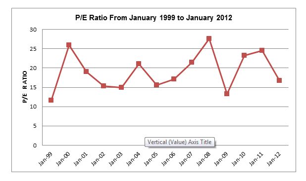
P/E ratio value for Nifty in January 1999 was around 11. It had started increasing and reached at the highest level of 26 in January 2000. In the year 2001, it remained steady between 18 and 20. In the year 2002, it started declining. In December 2002, P/E ratio declined below 14. Further in May 2003, Market turned to full circle and P/E ratio reached below the level of 1999. Then it again started rising and reached to 20 in December 2003. It again decreased to 1999 level in June 2004. From there it started rising and remained steady between 16 and 17 during 2005. It increased to the level of 20 during 2006 and 2007 and it reached the highest level of 28 in January 2008. From there it declines sharply to 13 in January 2009 and currently P/E is around 17 in January 2012.

The earlier empirical researches also indicate that low P/E securities tend to outperform high P/E securities. In short, Prices of securities are biased and a P/E ratio is an indicator of this bias. Paper also attempts to determine empirically whether the performance of equity shares are related to their P/E ratios. It shows that P/E phenomenon also exists in the Indian stock market.

Thus, macroeconomic variables and P/E ratio both plays a pivotal role in decision making for the investors. Therefore, study is divided into two parts. First part is about relationship between macroeconomic indicators and stock market returns. The second part is about low P/E securities inclined to outperform high P/E securities.

Limited numbers of papers have a discussion on macroeconomic variables and price-to-earnings ratio in Indian context for which review are mentioned as below.

Nelson (1976) examined the relationship between monthly stock returns and inflation in the post-war period from 1953 to 1974 using US data, and found a negative relationship between stock returns, in both expected and unexpected inflation.

The paper presented by Bodie (1976) defines the effectiveness of common stocks as an inflation hedge to the extent of which they can be used to reduce the risk of an investor’s real return which stems from uncertainty about the future level of the price of consumption goods.

Chen, Roll and Ross (1986) was the first study to select macroeconomic variables to estimate U.S. stock returns and apply the APT models. They employed seven macroeconomic variables, namely: term structure, industrial production, risk premium, inflation, market return, consumption and oil prices in the period of Jan 1953-Nov 1984. In their research, they found a strong relationship between the macroeconomic variables and the expected stock returns during the tested period. They note that industrial production, changes in risk premium, change in the yield curve, and unexpected changes in inflation during periods, when these variables are highly volatile. They found that stock returns are exposed to the systematic news and they were priced according to their exposure.

Clare and Thomas (1994) investigate the effect of 18 macroeconomic factors on stock returns in the U.K. They find oil prices, retail price index, bank lending and corporate default risk to be important risk factors for the U.K. stock returns.

Priestley (1996) pre-specified the elements that may carry a risk premium in the U.K. stock market. Seven macroeconomic and financial factors; namely default risk, industrial production, exchange rate, retail sales, money supply unexpected inflation, change in expected inflation, terms structure of interest rates, commodity prices and market portfolio. The APT model, with the factor generating from the rate of change approach all factors are important.

Naka, Atsuyuki; Mukherjee, Tarun; and Tufte, David (1998), analysed the relationship between macroeconomic variables and Indian stock market. To test the significance vector error correction model was used. The result indicates that inflation is severely restraining the performance of Indian stock market.

Flannery Mark J., Protopapadakis Aris A. (2002) stated in their research that the impact of macroeconomic variables on equity returns has been difficult to establish. CPI, Monetary Aggregate, Balance of Trade, Employment Report are the macro-economic variables were used for the study to identify the effect on equity returns. To establish the relevance GARCH model of daily equity returns and their conditionality volatility depends on macro series announcements. The study revealed that equity returns were significantly correlated with inflation and money growth.

Gay Robert D. (2008) explained in his research on effect of macroeconomic variables on stock market returns. He carried out the research on BRIC countries with two macroeconomic variables, viz., exchange rate and oil prices. He investigated the relationship using Box-Jenkins ARIMA model. Though he found no significant relationship between exchange rate and oil prices on stock market index prices but recognised that other domestic and international factors do affect the stock returns.

Ahmed (2010) has analysed the effect of macroeconomic variables on Turkish Stock Exchange Market in Arbitrage Pricing Theory framework. The author has studied seven macroeconomic variables (consumer price index, money market interest rate, gold price, industrial production index, oil price, foreign exchange rate and money supply) and the Turkish stock market Index. The author has studied for the time period of 2003 to 2010. He used multiple regression model to test the relationship. He found that interest rate, industrial production index, oil price, foreign exchange rate have negative effect on index returns while money supply positively influence the index returns.

Hassan, Gazi and Hisham, Al refai (2010) studied on the effect of macroeconomic factors on equity returns in long run. The researcher further found that trade surplus, foreign exchange reserves, money supply and oil prices are significant important macroeconomic variables which have long term effects on equity returns on Jordanian stock market. They have used regression approach and co-integration approach to study the significance. Both econometric methodologies found that macro-economic variables do have long-term effect on Jordanian stock market

Singh (2010) made an attempt to examine for Taiwan the casual relationship between index returns and certain crucial macroeconomic variable namely employment rate, exchange rate, GDP, Inflation and money supply. The analysis was based on stock portfolios rather than single stocks. The check the normality of data Kolmogorov-Smirnov D statistic normality test in SPSS 16 was performed. The author had applied regression to calculate the impact of macroeconomic variables on stock returns. The outcome of the study indicates that exchange rate and GDP seem to affect returns of all portfolios, while inflations rate, exchange rate and money supply have negative relationship with returns for portfolios.

Asaolu T.O., Ogunmuyiwa M.S. (2010) have investigated whether the effect of macroeconomic variables explain the changes in the stock price in Nigeria. He applied the econometric analysis by using the Augmented Dickey Fuller (ADF) test, Granger Casualty test, Co-integration and Error Correction method from the year 1986-2007. The outcome shows that the weak relationship has been identified between average stock prices and macro-economic variables. The macroeconomic variables considered for the study are inflation, interest rate, money supply and exchange rate.

Singh Dharmendra (2010) has explored the relationship considering the three macroeconomic variables, namely, wholesale price index, index of industrial production and exchange rate with BSE Sensex. He has applied correlation, unit root stationary test and Granger causality test. The author covered the time period from April, 1995 to March 2009 and concluded that Indian stock is information efficient with respect to exchange rate and inflation.

Izedonmi and Abdullahi (2011) have empirically tested the performance of Arbitrage Pricing Theory (APT) in the Nigerian Stock Exchange for the period of 2000 up to 2004 on monthly base. In the paper, they have identified three macroeconomic variables, (inflation, exchange rate and market capitalization) which are investigated against 20 sectors of Nigerian Stock Exchange. The authors have used the Ordinary Least Square (OLS) method and found that there are no significant effects of those variables in stock returns in Nigeria.

Hosseini, Ahmad and Lai (2011) studied the relationships between stock market indices and four macroeconomics variables, name crude oil price, money supply (M2), industrial production (IIP) and inflation rate in India and China. The study was made during January 1999 to January 2009. They have used unit root test of Augmented Dickey-Fuller, the underlying series are test as non-stationary at the level but stationary in first difference. They have also used Johansen-Juselius (1990) Multivariate Cointegration and Vector Error Correction Model, which indicate that there are both long and short run, linkages between the four selected macroeconomic variables and stock market indices in China and India. In long run, the impact of increasing crude oil price in China is positive but in India it is negative.

Naik Pramod, Padhi Puja (2012) have studied about the relationship of macroeconomic variables and stock market index. Five macroeconomic variables, namely, wholesale price index, money supply, treasury bills rates, exchange rate and industrial production index were taken into consideration to testify the relationship with stock market index. To signify the relationship Johansen’s co-integration and vector error correction model have been applied. They found that money supply and industrial production index are positively correlated with the stock market price but negatively correlated with inflation. The exchange rate and Treasury bill rates have insignificant relationship in determining the stock price.

Samadi Saeed, Bayani Ozra (2012) demonstrate that gold price, inflation and exchange rate have the influence on stock returns whereas oil price and liquidity has no impact on stock returns in Tehran stock market. The authors have assumed that data is stationery in nature and applied Augmented Dicky-Fuller (ADF) test.

Nicholson (1960) was first to demonstrate the P/E effect. He published a three page paper in which he included two studies. Data were taken from the statistical industry summaries prepared by Studley Shupert & Co. In the first study, he considered 100mainly industrial stocks over period from 1939 to 1959. He described that the lowest P/E quintile stock, rebalanced every five year, have delivered an investor 14.7 times his original investment at the end of 20 years as compared to 4.7 times for the highest P/E quintile stock. In the second study, he covered 29 Chemical Common stocks with prices and P/E ratios for the years 1937 to 1954. The 50% lowest P/E ratios averaged over 50% more appreciation than the 50% highest P/E ratios.

Nicholson (1968), in Nicholson extended his work by looking at the earnings of 189 companies between 1937 and 1962. Dividing companies into five groups by P/E ratios (P/E less than or equal to 10, P/E between 10 to 12, P/E between 12 to 15, P/E between 15 to 20, P/E greater than 20), he calculated mean price appreciation for each group. He found that the average price appreciation over seven years were 131% (12.71 % per annum) for companies with a P/E below ten, decreasing almost monotonically to71% (7.97% per annum) for those with P/E over 20. He concluded the purchase of the common stocks may logically seek the greater productivity represented by stocks with lower rather than higher P/E ratios.

Basu Sanjay (1977), described the relationship between common stocks and price-earnings ratio. In his research he has considered 14 year time period and establish that low P/E ratio portfolio earned 6% more per year than a high P/E portfolio. The stocks are ordered according to E/P ratio and divided into five equally weighted portfolios and re-ranked in January and rebalanced annually in April. The data was collected from NYSE and must have 60 months of data before it included in one of the five portfolios. He concluded that low P/E and high return relationship strictly increases from quintiles two to five. Average returns per annum were 9.34% for the highest P/E, with beta of 1.11, compared to 16.30% for the lowest P/E of 0.99. Basu recognised that the low P/E portfolios seem to have, on average, earned higher return than the high P/E securities.

A possible objection to Nicholson and Basu’s conclusions was made by Ball (1978). Ball argued that information available in the public domain at little or zero cost should not earn any private return. The marginal return from publicly available earning numbers should be zero. Ball looked at various possible explanations for this anomaly, including systematic experimental error, transaction and processing costs and failure of Sharpe’s two parameter CAPM model. In systematic experimental error, he included that most of the studies on announcements date assume announcement dates for all securities of 2 or 3 months after the fiscal period. Ball indicated that 25% of the firms did not announce within two months of the fiscal year end. Therefore, studies include some pre announcement and at announcement excess returns. This includes bias in the direction of anomaly. He also includes effect of shifts in securities’ relative risks upon estimated excess returns as a source of bias in anomaly. If relative risks are not independent of earnings or dividend yield, then experiments in which earnings or dividend yields vary across time or across securities could experience difficulty in controlling for risk.

Ball (1978), in explanation of transaction and processing cost, stated that investors attempting to act based on new information are handicapped because of transaction cost. Cost of processing earnings and dividend information are also very large. Such cost eliminated excess return. The contradict to this statement is proven by Joy, Litzen Berger, McEnally(1974), Watts(1971), Beaver (1975), Black(1973) and many other authors. They described that extreme rank earnings and dividend changes are associated with larger estimated excess return. Thus transactional and processing costs are not consistent with the observed variation in the excess return. Author also indicated that many variables such as relative risk of securities affect return of securities. These variables are not taken into consideration in many studies which used CAPM. Therefore, there exists a possible source of bias in anomaly.

Reinganum (1981) also claimed that simple, one period CAPM is miss-specified. The source of misspecification seems to be risk factors that are omitted from the CAPM as is evidence by the persistence of abnormal returns for at least two years. Data collected from issues of Wall Street journals and Compustat tapes were analysed in two distinct ways. The first was test of CAPM based on quarterly E/P ratios and the second was test of CAPM based on annual E/P ratio. In the first test, both pre and post announcement prices are used. Author constructed twenty securities portfolios (high E/P and low E/P) having estimated beta equal to one. Portfolio weights of individual securities are based upon the betas estimated with the sixty days of daily return data immediately preceding the three months holding period using an equal weighted NYSE-AMEX market index. Mean daily return difference between high P/E portfolio and low P/E portfolio was calculated. For the overall period, the difference was positive. Difference indicated that the high E/P (low P/E) portfolios have higher return than the low E/P (high P/E) portfolio. The similar analysis was repeated for firms having earning announcement in +2, +3 and +4 months after fiscal year. The excess return persisted for all the months. Therefore, author concluded that CAPM is miss-specified.

Similar study was repeated with annual data. In this test, securities were divided into 10 groups based on E/P value. Equal weights are applied to all securities. The equally weighted NYSE-AMEX market index was used as a control portfolio against which E/P portfolio returns were compared. Author concluded that CAPM is miss-specified since excess return persists for over two years. He also described that the high E/P (low P/E) portfolio has higher return than the low E/P (high P/E).

Reinganum also checked relationship of E/P and value anomalies (market value of firm). He used independent group method to form 25 portfolios. Mean excess return is defined as the daily return of EP-MV portfolio less the equal weighted NYSE-AMEX market daily return. Author observed that small firms in given E/P quintile outperform the high market value firms. The evidence did not weigh heavily in the favour of an E/P effect after controlling portfolio return for market value. Within low MV quintile, the lowest E/P securities possess a mean excess return greater than the high E/P securities. Thus, controlling ‘abnormal return’ for the value effect, an E/P effect is not detected. Thus value effect subsumes E/P effect.

Basu (1983) criticized Reinganum’s work on the grounds that he failed to adjust for risk and this caused him to underestimate earning yield effect. He claimed that E/P effect is significant even after controlling size effect.

Cook and Rozeff (1984) looked again to Reinganum’s and Basu’s findings in a more comprehensive statistical treatment, researching NYSE stocks from 1968 to 1981. Their paper provides joint tests for size and E/P effects using three different portfolio formulation rules (independent group, within group, within group with randomization). He used ANOVA for analysing effects. They found neither the size effect nor the E/P effect subsumes the other. They suggested that both effects are at work or they are separate aspect of single underlying effects.

Banz and Breen (1986) criticized all previous studies of size and P/E effects as suffering from two major biases (Ex-post selection bias and look-ahead bias). The ex-post selection bias meant that companies which had merged or gone bankrupt or otherwise disappeared did not appear in a commonly used COMPUSTAT database, and a new company appeared with a full accounting history that had not previously been available. The look-ahead bias means that portfolios were based on year-end accounting data that would not have been available to investors for several months more. Banz and Breen find that estimation of the E/P effect is not very sensitive to the ex-post selection bias but is quite sensitive to the look-ahead bias. Banz and Breen created their own database of 2500 securities (they have collected certain compustat items on monthly basis for several years) that accurately reflected the companies in existence and data available to investor at a time. Their sample period was January 1974 to December 1981. They created portfolios using within group method and tested hypothesis that the returns of this portfolios are different using different databases. They also tested relationship between E/P, size and return. They concluded that there is no relation between E/P and return as well as size and return by using their database. They attributed their findings to data source used. Their analysis suggests that much of the failure to account for the look-ahead bias can be avoided with the annual COMPUSTAT data by limiting the sample to December 31 fiscal closers and by computing E/P ratios using year-end earnings and March 31 prices.

Fuller, Huberts and Levinson (1993) did their best to disprove Ball’s arguments by including industry diversified portfolios for the out performance of low P/E shares. The study covers the period from 1973 to 1990. Only companies with an October, November, December, or January fiscal year-end are included in the sample. A minimum market capitalization screen is used to ensure that the stocks in the sample are representative of those from which institutional investors are likely to choose. CAPM model is used to calculate return on portfolio. In similarity to other studies, the author concluded that the high E/P securities generate higher excess return than the low E/P securities. Thus, the low P/E securities outperform the high P/E securities.M

Kane, Marcus and Noh (1996) examined the relationship between P/E, market volatility and the phase of the business cycle using market index data from 1954--1993. Dividend yield, the real interest rate, and the inflation rate are also included in the regression model. They used ARCH model for volatility measure instead of standard deviation because standard deviation is highly sensitive to outliers. They found that volatility, inflation rate and industrial production are negatively related to P/E, while the default premium is positively related to P/E.

White (2000) attempts to develop a tool to give some indication of when stocks have become priced irrationally high given a prevailing macroeconomic condition. Study includes past earnings growth, the inverse of the 10 year T-Bond yield, the 20-year T-Bond and dividend yields, inflation, real GDP growth, money supply, the total quarterly return on the S&P500, and the standard deviation of S&P500 monthly returns as independent variables in a time series regression study covering the period from 1926 to 1997. With E/P as the dependent variable, he finds negative coefficients for earnings growth, dividend pay-out, S&P500 total return and real GDP growth. Dividend yield, inflation, the 20-year T-Bond yield and the inverse of the 10-year T-Bond yield were positively related to E/P.

Yardeni (2003) indicates that perhaps the simplest attempt to model the determinants of P/E is Fed Model. This model indicates that the fair value of the market P/E (calculated using 12-month forward earnings. It is simply a time weighted average of the current and next years’ consensus estimates produced by Wall Street’s industry analysts) is the reciprocal of the ten-year Treasury bond yield. The logic behind this model is that stocks and bonds are competing assets and therefore a reduction in the bond yield should be associated with reductions in stock earnings yields. Yardeni also includes the second model for valuation by mentioning that Fed model was missing some of variables. The second model includes business risk to earnings and earnings expectations beyond the next 12 months.
E/P = CBY – (d x LTEG),

Where CBY is the current Moody’s A-rated corporate bond yield and LTEG is the consensus 5-year earnings growth forecast for the market index. The variable d is estimated from past data. Historically, d has had an average value of 0.13 over the period from 1985 to 2003. Asness (2003) argued that the Fed model is theoretically flawed because it compares a real number (E/P) to a nominal number (the bond yield). He describes three arguments in the favour of Fed model (The Competing Assets argument, The PV argument, Arguments based on data).The competing Assets argument says that Investor can either invest in stocks and bonds so they are competing assets. Comparison of Y and E/P is valid. The PV argument says that price of stock today has discounted present value of future cash flows to the investor from the company or market in question. It describes that when the interest rate falls the PV of future cash flow rises and so do fair P/Es. Fed model works for E/P and 10year treasury from 1965 to 2001. Asness has proved counter arguments against FED model using the Gordon model. In conclusion, Fed model seems to be successful in explaining how investors actually set current market P/E but it fails in forecasting long term returns.

Gupta, L. C., Jain, P. K., & Gupta, C. P. (1998), wrote a research monograph “Indian Stock Market P/E Ratios” which is a scientific guide to investors as well as policymakers. The book broadens and deepen the reader’s understanding of the Indian stock market. It provides very broad perspective on the market’s behaviour and pitfalls. It advocates the use of specially derived rule-of-thumb bench-mark P/E ratios for judging the state of the market. Analysis covers the period from 1980 to 1996. The study comprises two sets of partially overlapping analyses, one focusing on long term historical change in the P/E ratio from 1980 to 1994 and the other focusing on its short-term behaviour from 1990 to 1996.The long term historical analysis covers all those listed companies (broken down by size-classes) for which the required data was available in the Official Directory of the Bombay Stock Exchange. For short term behaviour, the sample was restricted to actively traded shares. Long term changes shows that the median P/E ratio was 6.6 for BSE National Index companies in the year 1979-80. It started rising in 1983 and reached a level of 13.4 in the year 1985. Thereafter, the ratio stabled around 12-13 for the rest of the 1980s. The main factor underlying the Indian stock market’s upward revaluation since mid-1980s was a policy induced rice in demand for equities among domestic investors, reinforced later by a gradual opening up of the market to overseas investors. The market gathers strong momentum during 1990s, leading to an unprecedented boom. However, by the mid-1990s, the market had turned full circle and collapsed. The demand based momentum in favour of equities as regards domestic investors had completely dissipated by the end of 1996. As a result Indian market underwent a substantial downward revaluation, pushing market P/E ratio below mid 1980s level.

Authors of the book also tried to provide bench marks for evaluating the Indian market’s average P/E ratio. Study to find relationship between P/E and company size (paid up equity capital, net worth and market cap) is also included by authors. The study also presents historical series of earning yield, divided yield and dividend pay-out ratio which are of considerable economic interest and are related to the P/E ratio.

Monica Singhania (2006) studied the various determinants of equity share prices with reference to Indian Stock market. The manufacturing companies listed on the BSE for which data is available on Prowess have been selected for analysis. Public sector companies were excluded as their policies are highly influenced by large number of social obligations and policy decision in the government, which may be difficult to account for. Financial (including banking) companies and utilities were also excluded because their strategic decisions are highly constrained by external forces including regulation. Regression method was used to find out relationships between Market price of equity and book value, dividend per share, earnings per share, dividend cover, growth, price earnings ratio and dividend yield. Result of analysis shows that price earning ratio, earning per share, book value and dividend cover are the variables which contributed the most in determining share prices followed by dividend per share and yield.

Ruzbeh J. Bodhanwala (2006) studied whether fund manager rely on quality of earnings and whether quality of earnings have correlation with market price of the share. The survey was conducted on 36 fund managers across 18 industries. Ten year data of 550 companies from Indian stock exchange have been selected for analysis. Ten portfolios have been constructed based on P/E, QE and B/M ratios. QE ratio was computed by dividing net profit after tax by cash flow from operating activities(Method for QE has been suggested by Warren Buffet and Martin Zweig. Sharpe measure has been used to calculate the return of the portfolio. The Sharpe returns of the portfolios are then compared with the excess market return over the risk free rate. The result suggests that the lowest P/E portfolio and the highest B/M portfolio outperformed the market. Although QE should be 1 but rarely it is so, from the portfolios it is evident that the best portfolios during the ten-year period are having QE in the range of 0.004- 1.212. This indicates that all companies whose market prices are increasing have more cash flow from operating activities in comparison to their net profit after tax. This is also indicative that the high amount of correlation exists between cash flow yield and market price.

Sultan Singh, Himani Sharma and Kapil Choudhary (2006) tested the semi strong efficient market hypothesis in Indian equity market by determining empirically whether the investment performance of common stocks is related to the investment strategies based on their P/E( Price-Earning ratio) and B/M (Book value to Market value ratio) ratios. S&P CNX 500 index has been chosen for data analysis. Securities were ranked according to the highest P/E ratio to the lowest P/E ratio. Five portfolios were formed based on P/E ratio. The continuously compounded returns of the portfolios were calculated assuming initial investment in each of their respective securities. Sharpe, Treynor and Jensen measures had been calculated to compare performance of the portfolios. The similar steps were performed on portfolios ranked based on B/M ratio. Author concluded that low P/E portfolios have earned the higher return than the high P/E portfolios and the high B/M portfolios have earned the higher return than the low B/M portfolios.

A. Vijayakumar, (2010), examined the extent to which financial performance indicators such as book value, earning per share , dividend per cover, growth rate and dividend yield affect the stock price. The study used correlation analysis, factor analysis and multiple linear regression to analyse the relationship. He established that all the variables have a positive association with the market price of Ashok Leyland and dividend per share and price-earnings ratio have negative association with the market price of its equity shares,

Much of the empirical studies of price-earnings ratio have been confined to US only. There exist very few studies in terms of Indian context in the area of price-earnings ratio. The literature discusses possible determinants of price-earnings ratio. The multivariate regression methodology has been used by most of the researchers to find relationship between macro-economic variables and stock market return. The studies indicate that inflation, exchange rate, oil prices, gross domestic product are all significantly correlated and plays the key role in determining the market price. Whereas money supply and interest rate show insignificant relationship with the market price. The literature also indicates that low price earning securities give better return to investor than high price- earnings ratio. There exist the controversy about size effect and price-earnings effect among few researchers which makes the study more interesting. The literature also discusses to major biases ex-post selection bias and look-ahead bias associated with most of the research based on financial data. Banz and Breen find that estimation of the earning-to-price ratio effect is not very sensitive to the ex-post selection bias but is quite sensitive to the look-ahead bias. They also gave solution for removing look-ahead biases. They suggested that earning-to-price ratios should be calculated using year-end earnings and March 31 prices. All the researches who did research afterwards on price-earnings ratio accepted their suggestion and calculated earning-to-price ratio by using year-end earnings and March 31 price.

REFERENCES :

1. Ahmed, E., Rosser Jr, J. B., & Uppal, J. Y. (2010). Emerging Markets and Stock Market Bubbles: Nonlinear Speculation?. Emerging Markets Finance and Trade, 46(4), 23-40.
2. Asaolu, T. O., & Ogunmuyiwa, M. S. (2011). An Econometric Analysis of the Impact of Macroeconomic Variables on Stock Market Movement in Nigeria. Asian Journal of Business Management, 3(1), 72-78.
3. Asness, C. (2003). Fight the Fed model: the relationship between stock market yields, bond market yields, and future returns. Bond Market Yields, and Future Returns (December 2002).
4. Ball R., (1978). “Anomalies in Relationships between securities’ yields and Yield-Surrogates”, Journal of Financial Economics, 6(2/3): 103-26.
5. Banz, R.W. and Breen, W.J., (1986). “Sample Dependent Results Using Accounting and Market Data: Some Evidence”, Journal of Finance, 41(4):779-93.
6. Basu S., (1975). “The Information Content of Price-Earnings Ratios”, Financial Management, 4(2): 53-64..
7. Basu S., (1977). “The Investment Performance of Common Stocks in relation to their Price-Earnings Ratios”, Journal of Finance, 32(3): 663-82.
8. Bhattacharya and Samanta, “Is the Spread between E/P Ratio and Interest Rate informative for Future Movement of Indian Stock Market?”, Paper No. 9, NSE
Research Paper.
9. Bodhanwala, R. J. (2005). An Empirical Study on Analysing How Fund Managers in India Analyse Financial Reports with Special Focus. Advances in Research in Business and Finance, 6, 33.
10. Bodie, Z. (1976). Common stocks as a hedge against inflation. The Journal of Finance, 31(2), 459-470.
11. Chan, L. K., Hamao, Y., & Lakonishok, J. (1991). Fundamentals and stock returns in Japan. The Journal of Finance, 46(5), 1739-1764.
12. Chen, N. F., Roll, R., & Ross, S. A. (1986). Economic forces and the stock market. Journal of business, 383-403.
13. Cook, T. J. and Rozeff, M. S., (1984). “Size and Earnings/ Price Ratio Anomalies: One Effect or Two?” Journal of Financial and Quantitative Analysis, 19(4): 449-66.
14. Desai, H., Rajgopal, S., & Venkatachalam, M. (2004). Value-glamour and accruals mispricing: One anomaly or two? The Accounting Review, 79(2), 355-385.
15. Fama, E. F., French, K. R. (1996). “Multifactor Explanations of Asset Pricing Anomalies.” Journal of Finance, 51, 55-84.
16. Flannery, M. J., & Protopapadakis, A. A. (2002). Macroeconomic factors do influence aggregate stock returns. Review of Financial Studies, 15(3), 751-782.
17. Gay Jr, R. D. (2011). Effect of macroeconomic variables on stock market returns for four emerging economies: Brazil, Russia, India, and China. International Business & Economics Research Journal (IBER), 7(3).
18. Gupta, L. C., Jain, P. K., & Gupta, C. P. (1998). Indian Stock Market P/E Ratios: A Scientific Guide to Investors and Policy Makers. Research Monograph, (6).
19. Gupta, L.C., Jain, P.K. and Gupta, C.P., (1998). “Indian Stock Market P/E Ratios: A Scientific Guide to Investors and Policymakers”, ISBN: 81-900513-5-0.
20. Hassan, G. M., & Al refai, H. M. (2012). Can macroeconomic factors explain equity returns in the long run? The case of Jordan. Applied Financial Economics, 22(13), 1029-1041.
21. Jain, P., & Rosett, J. (2001). Macroeconomic variables and the E/P ratio. P Ratio (December 15, 2001).
22. Kane, Marcus and Noh, (1996). “The P/E multiple and market Volatility”, Financial Analyst journal, July/August.M
23. Naka, A., Mukherjee, T., & Tufte, D. (1998). Macroeconomic variables and the performance of the Indian Stock Market.
24. Nicholson, S.F., (1960). “Price-Earnings Ratios”, Financial Analyst Journal, 16(4): 43-45.Nicholson, S.F., (1968). “Price-Earnings Ratios in relation to Investment Results”, Financial Analyst Journal, 24(1): 105-09.
25. Pramod Kumar, N., & Puja, P. (2012). The impact of Macroeconomic Fundamentals on Stock Prices revisited: An Evidence from Indian Data.
26. Priestley, R. (1996). The arbitrage pricing theory, macroeconomic and financial factors, and expectations generating processes. Journal of Banking & Finance, 20(5), 869-890.
27. Reinganum, M. R. (1981). Misspecification of capital asset pricing: Empirical anomalies based on earnings' yields and market values. Journal of financial Economics, 9(1), 19-46.
28. Samadi, S., Bayani, O., & Ghalandari, M. The Relationship between Macroeconomic Variables and Stock Returns in the Tehran Stock Exchange. International Journal, 2.
29. Singh, D. (2010). Causal relationship between macro-economic variables and stock market: a case study for India. Pakistan Journal of Social Sciences (PJSS), 30(2), 263-274.
30. Singhania Monica, (2006). “Determinants of Equity Prices: A study of select IndianCompanies”, the ICFAI Journal of Applied Finance, Vol. 12, No. 9, 39-50.
31. Sultan Singh, Himani Sharma and KapilChoudhary, (2006). “Performance of Equity in Relation to Fundamentals”, Financial Sector of India: Emerging Challenges, Ch 4, 60-72.
32. Vijayakumar, A. (2010). Effect of Financial Performance on Share Prices in the Indian Corporate Sector: An Empirical Study. Management and Labour Studies, 35(3), 369-381.
33. White, C. Barry. (2000). “What P/E Will the U.S. Stock Market Support?” FinancialAnalysts Journal, vol. 56, no. 6 (November/December): 30-38.
34. Yardeni, Edward. (2003). “Stock Valuation Models.” Prudential Financial Research, Topical Study no. 58: 2-30.