The similarity solution of Diffusion equation using a technique of infinitesimal transformations of groups
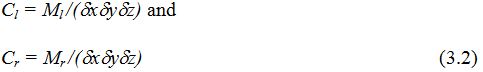
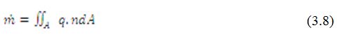
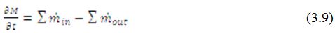
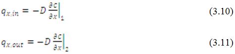
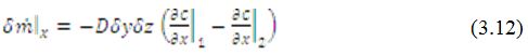
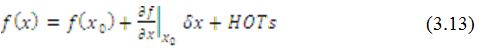
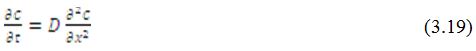
Abstract Keywords: Diffusion, Infinitesimal transformation, Similarity Solution. The diffusion equation describes the solute transport due to combined effect of diffusion and convection in a medium. It is a partial differential equation of parabolic type, derived on the principle of conservation of mass using Fick’s law. Due to the growing surface and subsurface hydroenvironment degradation and the air pollution, the diffusion equation has drawn significant attention of hydrologists, civil engineers and mathematicians. Its analytical/numerical solutions along with an initial condition and boundary conditions help to understand the contaminant concentration distribution behaviour through an open medium like air, rivers, lakes and porous medium like aquifer, on the basis of which remedial processes to reduce the damages may be enforced. It has wide applications in other disciplines too, like soil physics, petroleum engineering, chemical engineering and biosciences. Many researchers have discuss this problem from different aspects; for example, A.J.Janavicius and S.Turskiene[1] have obtained analytical solution of nonlinear diffusion equation; Nataliya M. Ivanova[2] has derived the exact solution of diffusion-convection equation. The systematical investigation of invariant solutions of different diffusion equation was started by the case of linear heat equation. (Miller W.[3] and Olver P.[4]). The infinite series solution of the diffusion equations are obtained by Carslow and Jaeger[5]; Crank[6] and others. In the mathematical theory of diffusion, the diffusion coefficient can be taken as constant in some cases, such as diffusion in dilute solution. In other cases, such as diffusion in high polymers, the diffusion coefficient depends on the concentrations of diffusing substance[6]. This paper presents similarity solution of one dimentional diffusion equation with constant diffusion coefficient. this solution is obtained by using a technique of infinitesimal transformations of groups. The solution obtained is physically consistant with results of earlier researchers and which is more classical than other results obtained by the earlier researchers. 2.0 Statement of the problem In order to evaluate how much of a chemical is present in any region of a fluid, we require a means to measure chemical intensity or presence. This fundamental quantity in environmental fluid mechanics is called concentration. In common usage, the term concentration expresses a measure of the amount of a substance within a mixture. A fundamental transport process in environmental fluid mechanics is diffusion. Diffusion differs from advection in that it is random in nature (does not necessarily follow a fluid particle). A well-known example is the diffusion of perfume in an empty room. If a bottle of perfume is opened and allowed to evaporate into the air, soon the whole room will be scented. We also know from experience that the scent will be stronger near the source and weaker as we move away, but fragrance molecules will have wondered throughout the room due to random molecular and turbulent motions. Thus, diffusion has two primary properties: it is random in nature, and transport is from regions of high concentration to low concentration, with an equilibrium state of uniform concentration. We just observed in our perfume example that regions of high concentration tend to spread into regions of low concentration under the action of diffusion. Here, we want to derive a mathematical expression that predicts this spreading-out process, and we will follow an argument presented in Fischer et al. [7]. To derive a diffusive flux equation, consider two rows of molecules side-by-side and centered at x = 0, Each of these molecules moves about randomly in response to the temperature (in a random process called Brownian motion). Here, for didactic purposes, we will consider only one component of their three-dimensional motion: motion right or left along the x-axis. We further define the mass of particles on the left as Ml, the mass of particles on the right as Mr, and the probability (transfer rate per time) that a particles moves across x = 0 as k, after some time 3.0 Mathematical formation Mathematically, the average flux of particles from the left-hand column to the right is kMl, and the average flux of particles from the right-hand column to the left is –kMr, where the minus sign is used to distinguish direction. Thus, the net flux of particles qx is For the one dimentional case, this equation can be written in terms of concentrations using where which gives, taking This equation contains two unknowns, k and Generalizing to three dimensions, we can write the diffusive flux vector at a point by adding the other two dimensions, Diffusion processes that obey this relationship are called Fickian diffusion, and above relation is called Fick’s law. To obtain the total mass flux rate we must integrate the normal component of q over a surface area, as in where n is the unit vector normal to the surface A. Although Fick’s law gives us an expression for the flux of mass due to the process of diffusion, we still require an equation that predicts the change in concentration of the diffusing mass over time at a point. In this section we will see that such an equation can be derived using the law of conservation of mass. To derive the diffusion equation, consider the control volume (CV) depicted in Figure 2. The change in mass M of dissolved tracer in this CV over time is given by the mass conservation law To compute the diffusive mass fluxes in and out of the CV, we use Fick’s law, which for the x-direction gives where the locations 1 and 2 are the inflow and outflow faces in the figure. To obtain total mass flux which is the x-direction contribution to the right-hand-side of (3.9). To continue we must find a method to evaluate ∂C/∂x at point 2. For this, we use linear Taylor series expansion, an important tool for linearly approximating functions. The general form of Taylor series expansion is
The similarity solution is obtained for one dimentional diffusion equation with constant diffusion coefficient. this solution is derived by using a technique of infinitesimal transformation of groups. The initial and boundary conditions are established for the diffusion coefficient to be constant. When these conditions are met, the diffusion coefficient can be easily evaluated.
Introduction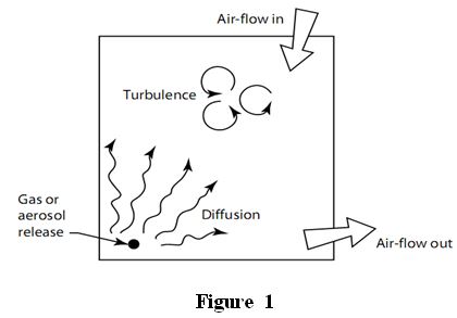
 an average of half of the particles have taken steps to the right and half have taken steps to the left.
 is the width,
  is the breadth, and
  is the height of each column. Physically, is the average step along the x-axis taken by a molecule in the time dt. For the one-dimensional case, we want qx to represent the flux in the x-direction per unit area perpendicular to x; hence, we will take = 1. Next, we note that a finite difference approximation for dC/dx is
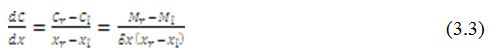
 =(xr-xr) , thus from (3.1) and (3.4), we have,
 , Fischer et al. [7] argue that since q cannot depend on an arbitrary , we must assume that k()2 is a constant, which we will call the diffusion coefficient, D. Substituting, we obtain the one-dimensional diffusive flux equation


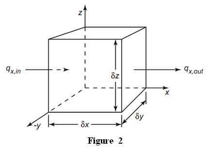
 we multiply qx by the CV surface area A =. Thus, we can write the net flux in the x-direction as
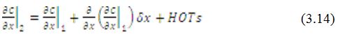
where HOTs stands for “higher order terms.” Substituting ∂C/∂x for f(x) in the Taylor series expansion yields
For linear Taylor series expansion, we ignore the HOTs. Substituting this expression into the net flux equation (3.12) and dropping the subscript 1, gives

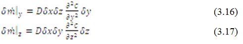
Similarly, in the y- and z-directions, the net fluxes through the control volume are
Before substituting these results into (1.19), we also convert M to concentration by recognizing M = C. After substitution of the concentration C and net fluxes  into (1.19), we obtain the three-dimensional diffusion equation
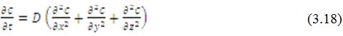
which is a fundamental equation in environmental fluid mechanics.
In the one-dimensional case, concentration gradients in the y- and z-direction are zero, and we have the one-dimensional diffusion equation
Where D is constatnt and called as diffusion coefficient.
4.0 Similarity SolutionWe consider all possible groups of infinitesimal transformation that will reduce the diffusion equation (3.19) to an ordinary differential equation. In applying such a technique to a given differential equation, it may turn out that for some or all of the groups other than the linear and spiral groups, the boundary condition cannot be transformed although the partial differential equation can be transformed into an ordinary differential equation. For such cases, we are at least assured that the groups of infinitesimal transformations that remain are the groups possible for the given boundary value problems. A similarity analysis of the diffusion equation from this point of view is apparently not covered in the literature. The one-dimensional form of the diffusion equation in rectangular coordinate is chosen because of its simplicity. Extension of analyses to equations expressed in other coordinates can readily be made.
Consider the diffusion equation 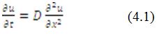
Where D is constant. On which an infinitesimal transformation is to be made on the dependent and independent variables and derivatives of the dependent variable with respect to the independent variable. The infinitesimal transformations are

Where generaters X, T and U are functions of x, t and u. Invarience of equation (1) under (2) gives
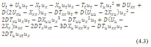
Equating to zero the coefficients of the corresponding terms, we get the following determining equations:
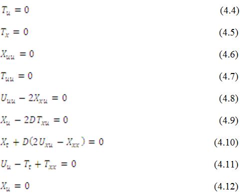
From these results, we conclude that,
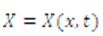

Now  , so
, so  function of x and t, also,

It follows that,
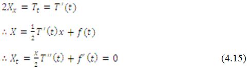
Now let 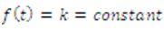 , then
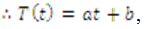 , a and b are constants
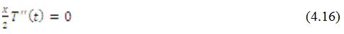
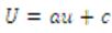 c is constant

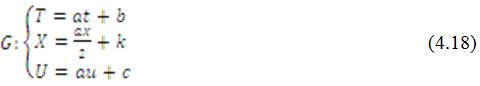
thus form equations (4.16), (4.17), the group G of inifinitesimal transformation explicitly is
The characteristic equations are
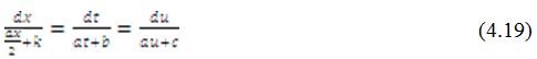
Let 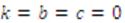 and
and , then from (4.19), we have,

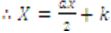
the first equation in (4.20) gives the similarity variable,

Now let , where
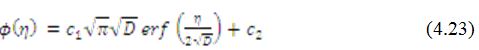
So, we get the second order ordinary differential equation,

Which is the second order linear ordinary differential equation and the general solution of the equation (4.22) is
5.0 Conclusion:
We have discussed here a specific problem of one dimentional diffusion equation under certain assumptions and obtained the similarity solution using the technique of a groups of infinitesimal transformations. We have expressed the solution in the form which is well suited for meaningful interpretation of the response of the physical problem. The numerical illustrations, although not discussed here due to our restrictive interest in the similarity study.
REFERENCES :
- A. J. Janavicius and S. Turskiene, Analytical solution of nonlinear diffusion equation in two dimentional surface, Acta physica polonica A, Vol 108 No. 6, 2005.
- Nataliya M. Ivanova, exact solution of diffusion-convection equation; Dynamics of PDE; Vol 5 No. 2; 139-171; (2008).
- Miller W.: Symmetry and separation of variable, reading, Addition-wesley, (1977).
- Olver P.: Applications of Lie groups of differential equations, New York, Springer-Verlag, (1986).
- H. S. Carslow and J. C. Jaeger: Conduction of heat in solids; Chap. 3, 2nd ed. Clarendon press, Oxford.(1959)).
- J. Crank: The Mathematics of Diffusion, Chap. 4, 2nd ed, Clarendon press, Oxford.(1975)
- H. B. Fischer, E. J. List, R. C. Y. Koh, J. Imberger and N. A. Brooks:Mixing in inland and coastal waters, Academic press, Inc., NY (1979).
- G. M. Murphy: Ordinary differential equations and their solutions, Van Nostrand reinhold company, NY.(1960), P 323.
***************************************************
K. J. Chauhan
Department of Mathematics,
Sir P. T. Sarvajanik College of Science,
Athwalines, Surat-395001, Gujarat-India.
Dr. D. M. Patel
Department of Mathematics,
Sir P. T. Sarvajanik College of Science,
Athwalines, Surat-395001, Gujarat-India.


Home | Archive | Advisory Committee | Contact us